'Newton's G-ball', marketed by Swedish company Mollic, is a simple electronic timing device which can be used to measure the freefall time from its point of release to impact on a surface below.
It is available from a number of third party suppliers, including djb microtech, Better Equipped and TIMSTAR in the UK and Arbor Scientific in the US.
 The ball has an integral centisecond timer, which is primed by pressing and holding the button on the face of the timer. Releasing the ball starts the timer, which stops when the ball impacts upon a surface below.
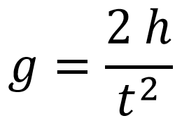
If the height, h, through which the ball falls is known, and the time for the ball to fall, t, is measured, then g can be calculated using the formula -
Taking multiple measurements of the freefall time, t, over a range of heights, h, allows a range of values to be obtained for g.
The results below were obtained by my Higher Physics class on 9th June 2016.
| h (m) | t1 | t2 | t3 | mean t (s) | g (ms-2) |
| 0.2 | 0.23 | 0.22 | 0.27 | 0.240 | 6.94 |
| 0.4 | 0.30 | 0.27 | 0.30 | 0.290 | 9.51 |
| 0.6 | 0.39 | 0.35 | 0.38 | 0.373 | 8.61 |
| 0.8 | 0.42 | 0.39 | 0.41 | 0.407 | 9.67 |
| 1.0 | 0.46 | 0.48 | 0.46 | 0.467 | 9.18 |
The results obtained are reasonably good, giving a mean value for g = 8.79 ms-2. Whilst this is in reasonably close agreement with the quoted value of 9.8 ms-2 given in the SQA data tables, discounting the obviously low value obtained for h = 0.2 m gives an improved mean value for g = 9.51 ms-2.
A quick analysis of the uncertainties in this data give the following -
Uncertainties in height, h (approximate reading/position uncertainty = ± 0.02 m)
| h (m) | uncertainty in h (m) | % uncertainty in h |
| 0.2 | 0.02 | 10% |
| 0.4 | 0.02 | 5% |
| 0.6 | 0.02 | 3% |
| 0.8 | 0.02 | 3% |
| 1.0 | 0.02 | 2% |
Uncertainties in time, t -
| h (m) | t1 | t2 | t3 | mean t (s) | random uncertainty in t (s) | % uncertainty in t |
| 0.2 | 0.23 | 0.22 | 0.27 | 0.240 | 0.017 | 7% |
| 0.4 | 0.30 | 0.27 | 0.30 | 0.290 | 0.010 | 3% |
| 0.6 | 0.39 | 0.35 | 0.38 | 0.373 | 0.013 | 4% |
| 0.8 | 0.42 | 0.39 | 0.41 | 0.407 | 0.010 | 2% |
| 1.0 | 0.46 | 0.48 | 0.46 | 0.467 | 0.007 | 1% |
Uncertainties in g -
| g (ms-2) | mean g
(ms-2) |
random uncertainty in g (ms-2) |
| 6.94 | 8.79 | 0.55 |
| 9.51 | ||
| 8.61 | % uncertainty in g | absolute uncertainty in g (ms-2) |
| 9.67 | 8% | 0.70 |
| 9.18 |
This gives a final value for g using this procedure as -
g = (8.79 ± 0.70) ms-2
However, an alternative graphical analysis allows an improved result to be obtained from the same data.
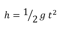
For this approach, the formula above was rearranged for h, giving -
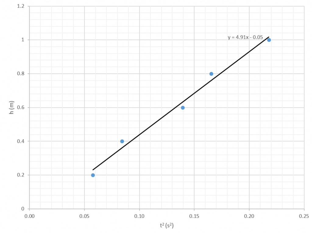
A graph was plotted of h against t2, giving a good approximation of a straight line through the origin, as expected.
| t2 (s2) | h (m) |
| 0.0576 | 0.2 |
| 0.0841 | 0.4 |
| 0.1394 | 0.6 |
| 0.1654 | 0.8 |
| 0.2178 | 1.0 |
Using the trendline function in Excel, a best fit line was added with its function included. The gradient of this straight line, which is equal to ½ g, is 4.91, giving a value for g from this graph - g = 9.82 ms-2.
Further analysis of the graph, using the LINEST function in excel, gave the following uncertainties -
| gradient | uncertainty in gradient | % uncertainty in gradient |
| 4.91 | 0.33 | 7% |
| g (ms-2) | absolute uncertainty in g (ms-2) |
| 9.82 | 0.69 |
This graphical treatment of the data gives a final value for g using this procedure as -
g = (9.82 ± 0.69) ms-2
I have included the raw data, graphical treatment and uncertainties in the in the excel file below.


G ball is also available from other uk suppliers such as Timstar.
Timstar now included in the list of suppliers. Thanks for letting me know.
And you can see it in use here: https://nustem.uk/activity/measuring-g/. Enjoy! ?